
Abstract
Introduction
A core feature that many users expect from their wearable devices is pulse rate estimation. Continuous pulse rate estimation can be informative for many aspects of a wearer’s health. Pulse rate during exercise can be a measure of workout intensity and resting heart rate is sometimes used as an overall measure of cardiovascular fitness.
Background
Physiological Mechanics of Pulse Rate Estimation
Pulse rate is typically estimated by using the PPG sensor. When the ventricles contract, the capillaries in the wrist fill with blood. The (typically green) light emitted by the PPG sensor is absorbed by red blood cells in these capillaries and the photodetector will see the drop in reflected light. When the blood returns to the heart, fewer red blood cells in the wrist absorb the light and the photodetector sees an increase in reflected light. The period of this oscillating waveform is the pulse rate.
Dataset
Data used for training is taken from TROIKA: A General Framework for Heart Rate Monitoring Using Wrist-Type Photoplethysmographic Signals During Intensive Physical Exercise.
12 subjects aged 18 to 35 were monitored as each subject ran on a treadmill with changing speeds for 5 minutes in this interval in their study In this study where the data was obtained there is also ground truth data provided which is gold standard since they collected the data.
- Sensors used to generate data
- ECG sensors
- PPG sensors
- Accelerometer sensors
Problem Statement
Build a pulse rate algorithm from the given dataset containing PPG and IMU signals that is robust to motion and “confidence metric” that estimates the accuracy of their pulse rate estimate. Then apply your algorithm to a new dataset to find more clinically meaningful features.
Zhilin Zhang, Zhouyue Pi, Benyuan Liu, ‘‘TROIKA: A General Framework for Heart Rate Monitoring Using Wrist-Type Photoplethysmographic Signals During Intensive Physical Exercise,’’IEEE Trans. on Biomedical Engineering, vol. 62, no. 2, pp. 522-531, February 2015. Link to Article
Analysis
Data Exploration
- what activities were performed in the dataset.
- features of the sensor that was used.
- the quantity of data in the dataset.
- short-comings of the dataset.
Algorithms and Techniques
Pulse Rate Algorithm
Code description
The code estimates pulse rate from PPG and acceleromter sensor signals. The ground truth pulse rate is taken from ECG signals measured contemporaneously.
Algorithm description
This algorithm uses signal data generated by the PPG sensors worn on a user’s wrist to estimate pulse rate.
The sensors emit light into a user’s wrist and detects the amount of light reflecting back to the PPG’s photodector.
The physiological aspect that a PPG measures is the amount of blood cells in one area. When the heart contracts, blood fills the extremities. When the heart relaxes, blood leaves the extremities and fill the heart.
PPG readings are high when the heart contracts and PPG readings are lower when the heart relaxes. The heart beats are typically a steady pulse rhythm, so these readings form a waveform whose period can be used to determine the pulse rate.
With the heart contractions, arm motions causes blood movement to the wrist. When running or walking, the arm movement can add another cadence to the PPG sensor measurements. The movements are periodic to separate these 3-axis accelerometers is used.
Sometimes, the strongest PPG frequency is the actual heart rate. However, the cadence of the arm swing is the same as the heartbeat. As a result, that PPG frequency is ruled out.
import glob
import os
import numpy as np
import scipy as sp
import scipy.io
import scipy.signal
import matplotlib.pyplot as plt
import pandas as pd
import matplotlib as mpl
import matplotlib.cm as cm

fs=125


def RunPulseRateAlgorithm(data_fl, ref_fl):
    """
     Estimates pulse rate

     Args:
        data_fl: (str) which is file path string to a troika.mat file with ECG, PPG, and ACC sensor datas.
        ref_fl:  (str) which is a file path to a troika.ma file with reference to heart rate

     Returns:
         errors: a numpy array of errors between pulse rate estimates and corresponding reference heart rates
         confidence: a numpy array of confidence estimates for each pulse rate.
    """

   # Load data using LoadTroikaDataFile
    ppg, accx, accy, accz = LoadTroikaDataFile(data_fl)

    # Compute pulse rate estimates

    #Load PPG and Accelerometer Signals.  Get Freqs and FFT Spectra for PPG and Accelerometer signals.
    fs=125
    nfft_window = fs*8
    noverlap = fs*6

    ppg_f = BandpassFilter(ppg)
    ppg_f_s, ppg_f_freqs,_,ppg_im = plt.specgram(ppg_f, NFFT = nfft_window, Fs=fs, noverlap=noverlap)
    plt.close()

    accx_f = BandpassFilter(accx)
    accx_s, accx_fqs,_,_ = plt.specgram(accx_f, NFFT = nfft_window, Fs=fs, noverlap=noverlap)
    plt.close()

    accy_f = BandpassFilter(accy)
    accy_s, accy_fqs,_,_ = plt.specgram(accy_f, NFFT = nfft_window, Fs=fs, noverlap=noverlap)
    plt.close()

    accz_f = BandpassFilter(accz)
    accz_s, accz_fqs,_,_ = plt.specgram(accz_f, NFFT = nfft_window, Fs=fs, noverlap=noverlap)
    plt.close()


    # Estimation confidence.

    max_f_ppg = []
    bpm_d = 10
    distance_bps = bpm_d/60
    count=0
    inner=0
    for i in range(ppg_f_s.shape[1]):
        accx_max_freq = accx_fqs[np.argmax(accx_s[:,i])]
        accy_max_freq = accy_fqs[np.argmax(accy_s[:,i])]
        accz_max_freq = accz_fqs[np.argmax(accz_s[:,i])]
        sorted_ppg_spcs = np.sort(ppg_f_s[:,i])[::-1]
        count += 1
        for f in range(10):
            ppg_freq = ppg_f_freqs[np.argwhere(ppg_f_s == (sorted_ppg_spcs[f]))[0][0]]
            inner+=1
            if ppg_freq == 0:
                continue
            elif (np.abs(ppg_freq-accx_max_freq)<=distance_bps) or (np.abs(ppg_freq-accy_max_freq)<=distance_bps) or (np.abs(ppg_freq-accz_max_freq)<=distance_bps):

                if f == 9:
                    max_f_ppg.append(ppg_f_freqs[np.argwhere(ppg_f_s == (sorted_ppg_spcs[0]))[0][0]])
                continue
            else:
                max_f_ppg.append(ppg_freq)
                break


    bpm_sum_window = 10
    bps_sum_window = bpm_sum_window/60

    ecgdata = sp.io.loadmat(ref_fl)['BPM0']

    confidences = []
    for i in range(ppg_f_s.shape[1]):
        low_window = max_f_ppg[i]-bps_sum_window
        high_window = max_f_ppg[i] + bps_sum_window
        window = (ppg_f_freqs>= low_window) & (ppg_f_freqs<=high_window)
        confidence=np.sum(ppg_f_s[:,i][window])/np.sum(ppg_f_s[:,i])
        error = np.abs(max_f_ppg[i]*60-ecgdata[i][0])
        confidences.append((i, max_f_ppg[i]*60, ecgdata[i][0], confidence, error))

    confidence_df = pd.DataFrame(
                    data=confidences,
                    columns=['WindowNumber','Estimated_Pulse_Rate','Ref_BPM','Confidence','Error'])

    # Return per-estimate mean absolute error and confidence as a 2-tuple of numpy arrays.

    errors = confidence_df['Error'].values
    confidence = confidence_df['Confidence'].values

    return errors, confidence
Methodology
Data Processing and Visualization
fs = 125
window = 2
ds, ref = LoadTroikaDataset()
ds1 = ds[0]
ds1 = LoadTroikaDataFile(ds1)
ds1
ppg, accx, accy, accz = ds1
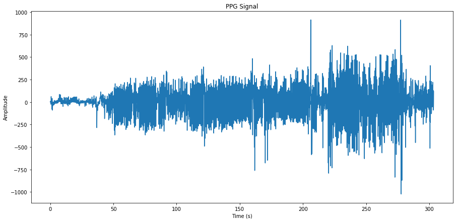
ts = np.arange(0,len(ppg)/fs,1/fs)
plt.figure(figsize=(15,7))
plt.plot(ts,ppg)
plt.title("PPG Signal")
plt.xlabel("Time (s)")
plt.ylabel("Amplitude")
plt.show()
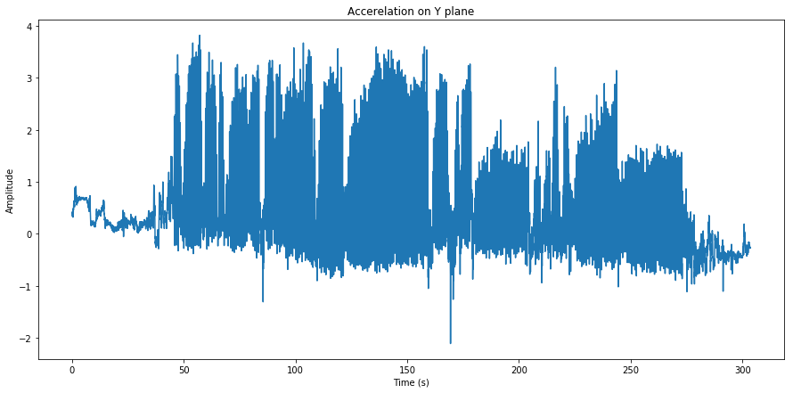
ppg, accx, accy, accz = ds1
ts = np.arange(0,len(accx)/fs,1/fs)
plt.figure(figsize=(15,7))
plt.plot(ts,accx)
plt.title("Accerelation on X plane")
plt.xlabel("Time (s)")
plt.ylabel("Amplitude")
plt.show()
Results
Algorithm Performance
fs = 125
data_list = [ppg, accx, accy, accz]
label_list = ['ppg', 'accx', 'accy', 'accz']

filtered = {label : BandpassFilter(data) for (label, data) in zip(label_list, data_list)}
ppg_sig = filtered['ppg'][1000:2000]
pks = sp.signal.find_peaks(ppg_sig, height=15, distance=35)[0]

fig, ax1 = plt.subplots(figsize=(16, 10))
ax2 = ax1.twinx()

ax1.plot(ppg_sig, 'black')
ax1.plot(pks, ppg_sig[pks], 'r.', ms=10)

for label in label_list[1:]:
    ax2.plot(filtered[label][1000:2000], label=label)
    ax2.legend(loc='upper right')

plt.show()
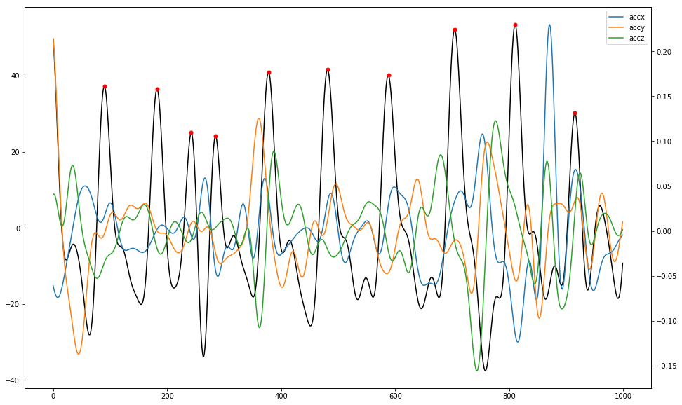
Characteristic frequencies for the PPG data is compared against the dominant characteristic frequencies for each accelerometer axis per time window.
The Confidence of each frequency’s determination is calulated as intensity magnitudes near the charactistic frequncy divided by the sum of intensity magnitudes across all frequencies. This method to calculate confidence is similar to Signal to Noise ratio calculation, where a higher result indicates fewer noise frequencies that are not characteristic of the pulse rate. One may select BPM estimates above a threshold confidence while discarding those below the threshold.
The Absolute Errors are calculated between the determined PPG frequency and the reference ECG pulse rate data. The output from this algorithm only takes into account arm movement noise that is periodic. It doesn’t remove non-periodic movements. This algorithm also doesn’t account for other noise sources such as ambient light or shifts in sensor position.
Clinical Application
For clinical Application the data this phase comes from the Cardiac Arrythmia Suppression Trial (CAST), which was sponsored by the National Heart, Lung, and Blood Institute (NHLBI). CAST collected 24 hours of heart rate data from ECGs from people who have had a myocardial infarction (MI) within the past two years.[1] This data has been smoothed and resampled to more closely resemble PPG-derived pulse rate data from a wrist wearable.[2]
CAST RR Interval Sub-Study Database Citation - Stein PK, Domitrovich PP, Kleiger RE, Schechtman KB, Rottman JN. Clinical and demographic determinants of heart rate variability in patients post myocardial infarction: insights from the Cardiac Arrhythmia Suppression Trial (CAST). Clin Cardiol 23(3):187-94; 2000 (Mar)
Physionet Citation - Goldberger AL, Amaral LAN, Glass L, Hausdorff JM, Ivanov PCh, Mark RG, Mietus JE, Moody GB, Peng C-K, Stanley HE. PhysioBank, PhysioToolkit, and PhysioNet: Components of a New Research Resource for Complex Physiologic Signals (2003). Circulation. 101(23):e215-e220.
metadata.head()

  subject age sex
0 e198a 20-24 Male
1 e198b 20-24 Male
2 e028b 30-34 Male
3 e028a 30-34 Male
4 e061b 30-34 Male
metadata.describe()

        subject age sex
count   1543  1543  1543
unique  1543  11  2
top     e195b 60-64 Male
freq     1    313   he1266
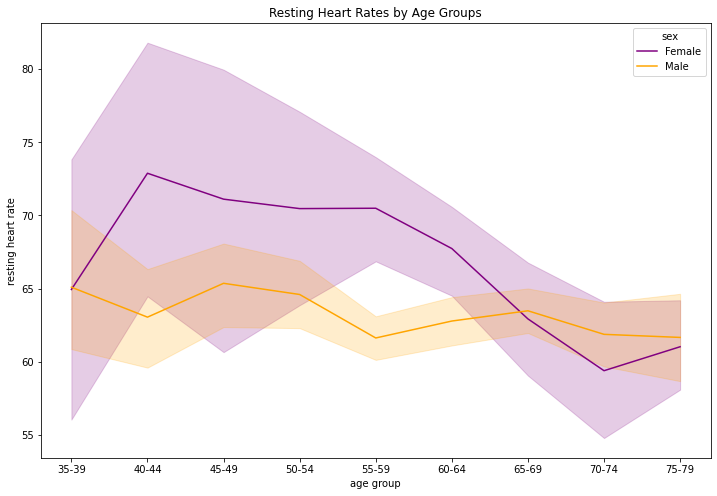
Clinical Conclusion
- For women, we see dropping with the age 70 to
- For men, we see from age 60 to 69 there are more male of this age category
- In comparison to men, women’s heart rate is higher compared to the male
- With 1543 participants I would say the sample size good.
- There sholud be younger age also
Conclusion
As wearables become more widespread in medical research, these kinds of analyses can play a large part in the discovery process. With large enough datasets and more informative clinical metadata (in this case, we only used age group), wearables can be used to discover previously unknown phenomena that may advance clinical science.
Before doing any analysis, however, engineers and data scientists will have to process the large amounts of raw data that wearables collect.