
Abstract
Atrial Fibrillation
Atrial fibrillation (AFib) is a condition where the heartbeat becomes erratic and the upper chambers of the heart quiver and shake. If there’s a lurking blood clot, this shaking can break it loose and send it up through the blood vessels to the brain, where it can cause a stroke. People with AFib have a 5 times greater likelihood of having a stroke, and doctors typically put patients with the condition on blood-thinning medications that prevent clots. Article
- Arrhythmia: An irregular heart rhythm.
- Sinus Rhythm: The normal, regular heart rhythm, paced by the sinus node.
- Atrial fibrillation: An irregular rhythm caused by multiple, haphazard depolarizations across the atria.
- Behar, Rosenberg, Yaniv, Oster. Rhythm and Quality Classification from Short ECGs Recorded Using a Mobile Device. Computing in Cardiology Challenge 2017.
- Bonizzi, Driessens, Karel. Detection of Atrial Fibrillation Episodes from Short Single Lead Recordings by Means of Ensemble Learning. Computing in Cardiology Challenge 2017.
Background
The heart is made up of four chambers, two atria and two ventricles. The atria pump blood into the ventricles and then the ventricles pump blood throughout the body. Each heart cell is polarized, meaning there is a different electrical charge inside and outside of the cell. At rest, the inside of the cell is negatively charged compared to the outside. When the cell depolarizes, positive charges outside of the cell flow inside and makes the interior of the cell positively charged relative to the outside. This depolarization causes the cell to contract. The movement of charges across a heart cell’s membrane is the source of the electrical activity that gets measured by an ECG.
The conduction of electrical impulses through the heart follows a regular pattern orchestrated by the cardiac conduction system. Each heartbeat starts with an impulse in the sinus (SA) node. The sinus node is the natural pacemaker of the heart and is responsible for setting the heart’s natural rhythm. The impulse then propagates throughout the atria and causes the atria to contract. Then, the impulse enters the atrioventricular (AV) node, which delays the propagation of the signal to the ventricles. This gives the atria time to pump blood into the ventricles. After a brief pause, the signal passes through the AV node and into the ventricles, causing the ventricles to contract. This is the largest electrical disturbance in the cardiac cycle. After the ventricles contract, they repolarize, meaning the ions move back across the cell wall to their initial resting state.
Each part of this sequence is responsible for creating a distinct marker– or wave –in the ECG signal. The P-wave corresponds to the depolarization of the atria. The pause between the P-wave and the Q-wave is caused by the AV node delaying the electrical impulse to the ventricles. When the ventricles contract, we see the large QRS complex. And finally, after some time, the ventricles repolarize, causing the T-wave. The atria repolarize around the same time as the ventricles finish contracting so that activity is not visible in an ECG because it is obscured by the S-wave.
This cycle repeats every heartbeat and results in a very regular and uniform looking signal.

Dataset
The data we will use comes from the Computing in Cardiology (CinC) Challenge 2017 dataset hosted on Physionet.
The dataset contains thousands of short ECG snippets (30s - 60s) from the AliveCor mobile ECG monitor. The original challenge was to build a 4-class classifier for sinus rhythm, atrial fibrillation, alternative rhythm, and noisy record. We will throw out the noisy records and build a two-class classifier distinguishing between sinus rhythm and another rhythm (atrial fibrillation included).link to dataset
Problem Statement
Build a two-class classifier distinguishing between sinus rhythm and another rhythm (atrial fibrillation included).
Metrics
We will use confusion matrix. Confusion matrix is a very popular measure used while solving classification problems. It can be applied to binary classification as well as for multiclass classification problems.
The confusion matrix, also known as the error matrix, is depicted by a matrix describing the performance of a classification model on a set of test data.
Confusion matrices represent counts from predicted and actual values. The output TN stands for True Negative which shows the number of negative examples classified accurately. Similarly, TP stands for True Positive which indicates the number of positive examples classified accurately. The term FP shows False Positive value, i.e., the number of actual negative examples classified as positive; and FN means a False Negative value which is the number of actual positive examples classified as negative. One of the most commonly used metrics while performing classification is accuracy. The accuracy of a model (through a confusion matrix) is calculated using the given formula below.
Accuracy =    TN + TP
           ----------------
           TN + FP + FN + TP
Accuracy can be misleading if used with imbalanced datasets, and therefore there are other metrics based on confusion matrix which can be useful for evaluating performance. In Python, confusion matrix can be obtained using confusion_matrix() function which is a part of sklearn library. This function can be imported into Python using from sklearn.metrics import confusion_matrix. To obtain confusion matrix, users need to provide actual values and predicted values to the function
Analysis
Data Exploration
We use reference data. Reference data is a flat table that tells us what rhythm each record is in. N for normal sinus rhythm and O for other rhythm. Our task will be to classify ECG signals into these two classes.
ref.head()

record  rhythm
0 A00001  N
1 A00002  N
2 A00003  N
3 A00004  O
4 A00005  O
ref.rhythm.value_counts()

N    4529
O    2887
Name: rhythm, dtype: int64
We have roughly 1.5x more sinus rhythm data than other.
Exploratory Visualization
Let’s take a look at how long each ECG record is. The sampling rate for this dataset is 300 HZ
fs = 300
plt.figure(figsize=(10, 6))
plt.hist(np.array(list(map(len, ecgs))) / fs);
plt.xlabel('Time (sec)')
plt.title('Length of ECG records')

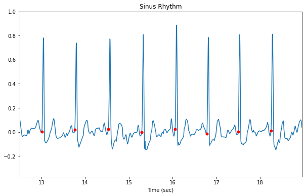
Now let’s look at the raw ECG data plotted with the QRS locations.
Normal sinus rhythm
By looking at sinus rhythm data we can get a sense of the noise level in the sensor without dealing with rhythm-induced artifacts.
plt.figure(figsize=(10, 6))
ecg, qrs = ecgs[0], qrs_inds[0]
ts = np.arange(len(ecg)) / fs
plt.plot(ts, ecg)
plt.plot(ts[qrs], ecg[qrs], 'r.', ms=10, label='QRS Detections')
plt.xlim((12.5, 18.95))
plt.xlabel('Time (sec)')
plt.ylim((-.37, 1))
plt.title('Sinus Rhythm')
Noisy sinus rythm
Sometimes our ECG rhythm will be interrupted by transient noise artifacts, most likely caused by user error or motion artifact. Even in the presence of motion, the QRS detection algorithm still finds QRS complexes. In the presence of noise, there surely might be some error in the QRS detections.
plt.figure(figsize=(10, 6))
ecg, qrs = ecgs[1], qrs_inds[1]
ts = np.arange(len(ecg)) / fs
plt.plot(ts, ecg)
plt.plot(ts[qrs], ecg[qrs], 'r.', ms=10, label='QRS Detections')
plt.xlim((16.74, 20.91))
plt.xlabel('Time (sec)')
plt.ylim((-0.68, 1.74))
plt.title('Noisy Sinus Rhythm')

Algorithms and Techniques
Features
The features for the AF detection algorithm are computed from the RR interval time series. We use the time domain and frequency domain features listed below.
Time domain
- minimum RR interval
- maximum RR interval
- median RR interval
- average RR interval
- standard deviation of RR intervals
- number of RR interval outliers
- An RR interval is an outlier if it is greater than 1.2x the average RR interval in the ECG record
- root-mean-square of the difference between adjacent RR intervals
- percent of RR interval differences greater than 50 milliseconds
Frequency domain
The RR interval time series is not sampled regularly in time. We only have a datapoint every heart beat. Before we can compute any frequency domain features, the time series must be resampled so that we get uniform data points. Resample the RR interval time series to 4 Hz before computing the features below.
- peak magnitude between 0.04 Hz and 0.15 Hz in the regularized RR interval time series
- main frequency between 0.04 Hz and 0.15 Hz in the regularized RR interval time series
- peak magnitude between 0.15 Hz and 0.4 Hz in the regularized RR interval time series
- main frequency between 0.15 Hz and 0.4 Hz in the regularized RR interval time series
Implementation
def Featurize(qrs_inds, fs):
   """Featurize the qrs complex locations time series.

   Args:
       qrs_inds: (np.array of number) the sample indices of the QRS complex locations
       fs: (number) the sampling rate

   Returns:
       n-tuple of features
   """
   # Compute the RR interval time series
   rr = np.diff(qrs_inds)

   # Compute time domain features
   if len(qrs_inds) < 1:
       return [0,0,0,0,0,0,0,0,0,0,0,0]
   else:
       pass
   min_rr = np.min(rr)
   max_rr = np.max(rr)
   median_rr = np.median(rr)
   mean_rr = np.mean(rr)
   std_rr = np.std(rr)
   n_outliers = np.sum(rr > 1.2 * np.mean(rr))
   rmssd = np.sqrt(np.mean(np.square(np.diff(rr))))
   pdrr_50 = np.mean(np.diff(rr) / fs > 0.05)

   # Regularly resample the RR interval time series
   rr_ts = np.arange(qrs_inds[0] / fs, qrs_inds[-2] / fs, 1 / 4)
   rr_interp = np.interp(rr_ts, qrs_inds[:-1] / fs, rr)

   # Compute the Fourier transform of the regular RR interval time series
   freq = np.fft.rfftfreq(len(rr_interp), 1 / 4)
   fft_mag = np.abs(np.fft.rfft(rr_interp))

   # Compute frequency domain features
   lf_mag = np.max(fft_mag[(freq >= 0.04) & (freq <= 0.15)])
   lf_freq = freq[np.argmax(fft_mag[(freq >= 0.04) & (freq <= 0.15)])]
   hf_mag = np.max(fft_mag[(freq >= 0.15) & (freq <= 0.4)])
   hf_freq = freq[np.argmax(fft_mag[(freq >= 0.15) & (freq <= 0.4)])]


   return (min_rr, max_rr, median_rr, n_outliers, mean_rr, std_rr, rmssd, pdrr_50,
           lf_mag, lf_freq, hf_mag, hf_freq)
Create Feature Matrix
feats = [Featurize(qrs_inds, fs) for qrs_inds in qrs]
X, y = np.array(feats), np.array(labels)
Train
We will train by building a Classfier to classify our ECG records. a random forest with 100 trees and a depth of 4 works well.
Lastly we evaluate the performance of the classifier using cross validation.
from sklearn.ensemble import RandomForestClassifier
from sklearn.model_selection import KFold
from sklearn.metrics import confusion_matrix

# Use A RandomForestClassifier

clf = RandomForestClassifier(n_estimators=100,
                             max_depth=4,
                             random_state=0,
                             class_weight='balanced')

# Evaluate with 7-fold cross validation
cv = KFold(7, shuffle=True, random_state=0)

# Keep an aggregated confusion matrix
cm = np.zeros((2,2), dtype='int')

# As well as aggregated predictions with labels
y_tests = []
y_preds = []

for train_ind, test_ind in cv.split(X, y):
    # Subset dataset
    X_train, y_train = X[train_ind], y[train_ind]
    X_test, y_test = X[test_ind], y[test_ind]

    # Train model
    clf.fit(X_train, y_train)

    # Run model
    y_pred = clf.predict(X_test)

    # Aggregate results
    y_tests.append(y_test)
    y_preds.append(y_pred)
    cm += confusion_matrix(y_test, y_pred, labels=['O', 'N'])
Evaluate
Compute Performance Metrics
We will evaluate the classfier performance by computing precision and recall on detecting no-sinus(other) rhythm
Using aggregated predictions and labels
From a vector of all predictions and the correct labels, we can use numpy operations to count the number of true positives, false positives, and false negatives. We can then use this to compute and recall
yt = np.hstack(y_tests)
yp = np.hstack(y_preds)
tp = np.sum((yp == 'O') & (yt == 'O'))
fp = np.sum((yp == 'O') & (yt == 'N'))
fn = np.sum((yp == 'N') & (yt == 'O'))
precision = tp / (tp + fp)
recall = tp / (tp + fn)
precision, recall

(0.72606135729779986, 0.81156910287495665)
Using the confusion matrix
We can also get the number of true positves, false positives, and false negatives directly from the confusion matrix to compute precison and recall
tp = cm[0, 0]
fp =  cm[1, 0]
fn = cm[0, 1]
precision = tp / (tp + fp)
recall = tp / (tp + fn)
precision, recall

(0.72606135729779986, 0.81156910287495665)
Summary
I used a RandomForestClassifier with 100 trees and a max depth of 4. With these basic features, it achieved a precision of 73% and a recall of 81%. Further improvements can be made by using a more advanced technique for RR interval time series regularization, and by using more informative features.