
Abstract
Bike-sharing demand is highly relevant to related problems companies encounter, such as Uber, Lyft, and DoorDash. Predicting demand not only helps businesses prepare for spikes in their services but also improves customer experience by limiting delays
Project Environment
AWS Sagemaker Studio was used for this project as it can be seen in the project repo.
Data set
Data was downloaded from kaggle.
!kaggle competitions download -c bike-sharing-demand
!unzip -o bike-sharing-demand.zip
Problem Statement
Predict Bike Sharing Demand with AutoGluon AutoML
Initial Training
Initial training is used as benchmark for further training to see if there will be changes on model performance. The training is done using Automl. The algorithm used is AutoGluon.
We are predicting count, so it is the label we are setting.
- Ignore casual and registered columns as they are also not present in the test dataset.
- Use the root_mean_squared_error as the metric to use for evaluation.
- Set a time limit of 10 minutes (600 seconds). Use the preset best_quality to focus on creating the best model.
predictor = TabularPredictor(label="count",
                             eval_metric='root_mean_squared_error',
                             problem_type='regression',
                             learner_kwargs={'ignored_columns': ['casual','registered']}
                            ).fit(train_data=train,
                                  time_limit=600,
                                  presets="best_quality"
)
The number of models which were trained were 15, in this stage there was no data preprocessing.
Estimated performance of each model:
                     model   score_val  pred_time_val    fit_time  pred_time_val_marginal  fit_time_marginal  stack_level  can_infer  fit_order
0      WeightedEnsemble_L3  -52.847596      11.249226  502.330480                0.001120           0.436674            3       True         15
1   RandomForestMSE_BAG_L2  -53.473435      10.375775  403.099560                0.597212          25.713495            2       True         12
2     ExtraTreesMSE_BAG_L2  -53.810409      10.386975  385.264302                0.608412           7.878237            2       True         14
3          LightGBM_BAG_L2  -55.046580       9.989433  398.853544                0.210870          21.467479            2       True         11
4          CatBoost_BAG_L2  -55.516287       9.831613  446.834595                0.053049          69.448530            2       True         13
5        LightGBMXT_BAG_L2  -60.425971      13.133647  427.012202                3.355083          49.626137            2       True         10
6    KNeighborsDist_BAG_L1  -84.125061       0.038490    0.029288                0.038490           0.029288            1       True          2
7      WeightedEnsemble_L2  -84.125061       0.039427    0.675935                0.000937           0.646647            2       True          9
8    KNeighborsUnif_BAG_L1 -101.546199       0.038787    0.031544                0.038787           0.031544            1       True          1
9   RandomForestMSE_BAG_L1 -116.544294       0.534120   10.116589                0.534120          10.116589            1       True          5
10    ExtraTreesMSE_BAG_L1 -124.588053       0.530154    4.933934                0.530154           4.933934            1       True          7
11         CatBoost_BAG_L1 -130.482869       0.099427  191.457479                0.099427         191.457479            1       True          6
12         LightGBM_BAG_L1 -131.054162       1.488921   25.595079                1.488921          25.595079            1       True          4
13       LightGBMXT_BAG_L1 -131.460909       6.707506   59.929166                6.707506          59.929166            1       True          3
14  NeuralNetFastAI_BAG_L1 -136.015060       0.341158   85.292985                0.341158          85.292985            1       True          8
Number of models trained: 15
Best model was "WeightedEnsemble_L3"
The top ranked model that performed
The best top ranked model in Initial training was “WeightedEnsemble_L3”
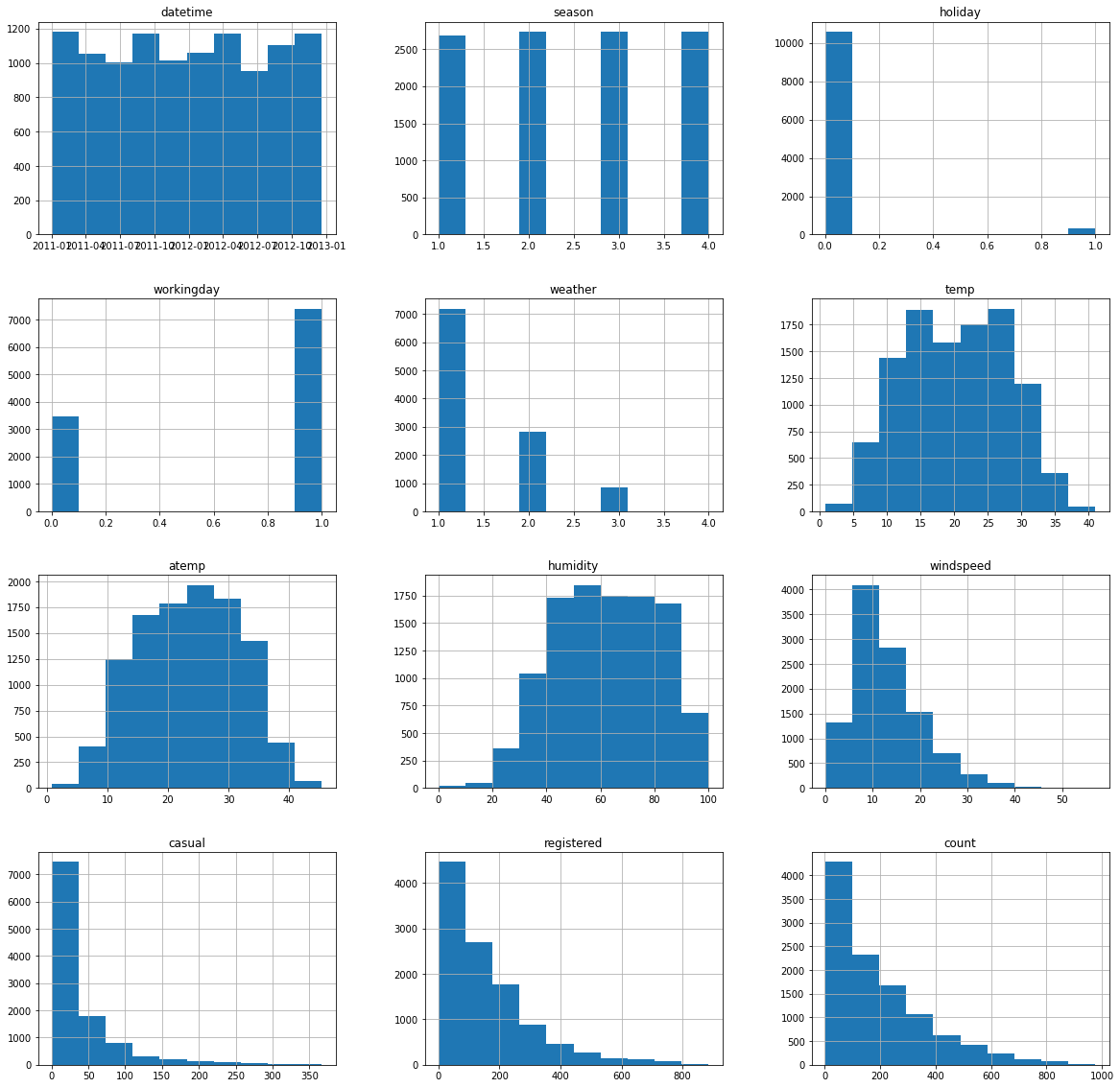
ETL
DataFrame.describe() pandas method generates descriptive statistics that summarize the central tendency, dispersion and shape of a dataset’s distribution, excluding NaN values. This method tells us a lot of things about a dataset. One important thing is that the describe() method deals only with numeric values. It doesn’t work with any categorical values. So if there are any categorical values in a column the describe() method will ignore it and display summary for the other columns unless parameter include=“all” is passed.
- count tells us the number of Non-empty rows in a feature.
- mean tells us the mean value of that feature.
- std tells us the Standard Deviation Value of that feature.
- min tells us the minimum value of that feature.
- 25%, 50%, and 75% are the percentile/quartile of each features. This quartile information helps us to detect Outliers.
- max tells us the maximum value of that feature.
The snipet below shows the summary of the describe function and also the information about the dataset
            count   mean      std       min   25%     50%   75%      max
season      10886.0 2.506614  1.116174  1.00  2.0000  3.000 4.0000  4.0000
holiday     10886.0 0.028569  0.166599  0.00  0.0000  0.000 0.0000  1.0000
workingday  10886.0 0.680875  0.466159  0.00  0.0000  1.000 1.0000  1.0000
weather     10886.0 1.418427  0.633839  1.00  1.0000  1.000 2.0000  4.0000
temp        10886.0 20.230860 7.791590  0.82  13.9400 20.500  26.2400 41.0000
atemp       10886.0 23.655084 8.474601  0.76  16.6650 24.240  31.0600 45.4550
humidity    10886.0 61.886460 19.245033 0.00  47.0000 62.000  77.0000 100.0000
windspeed   10886.0 12.799395 8.164537  0.00  7.0015  12.998  16.9979 56.9969
casual      10886.0 36.021955 49.960477 0.00  4.0000  17.000  49.0000 367.0000
registered  10886.0 155.552177 151.039033 0.00  36.0000 118.000 222.0000  886.0000
count       10886.0 191.574132 181.144454 1.00 42.0000 145.000 284.0000  977.0000
Feature engineering
Transforming the weather and season columns to category from ints since autogluon sees them as ints. Parsing the datetime to separate features for further analyis
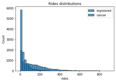
Ride distribution for registered and unregistered users
The registered users perform way more rides than casual ones. Furthermore, we can see that the two distributions are skewed to the right, meaning that, for most of the entries in the data, zero or a small number of rides. Finally, every entry in the data has quite a large number of rides (that is, higher than 800).
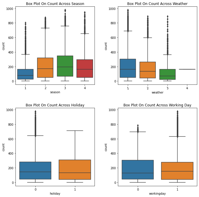
Average of bike using accross the Year
The average of using bikes accross seasons, accross weather, working day and holiday.
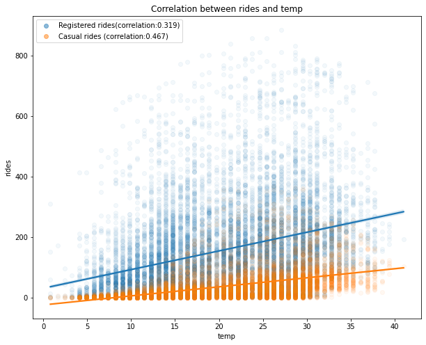
Plotting Correlations
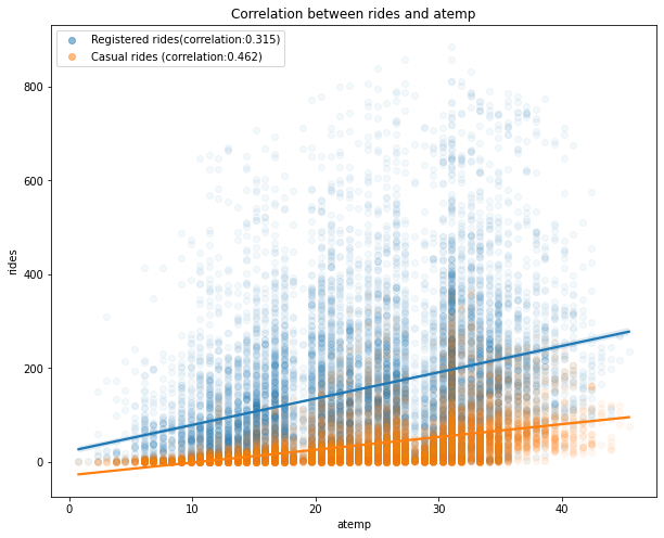
Correlation between rides and temperature . The higher temperatures have a positive impact on the number of rides (the correlation between registered/casual rides and temp is 0.32 and 0.46, respectively, and it’s a similar case for atemp). Note that as the values in the registered column are widely spread with respect to the different values in temp, we have a lower correlation compared to the casual column.
Correlation between rides and temperature
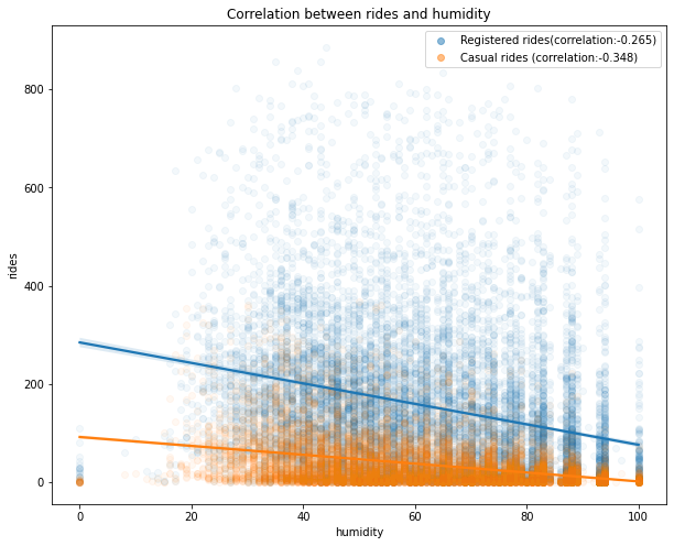
Correlation between rides and humidity
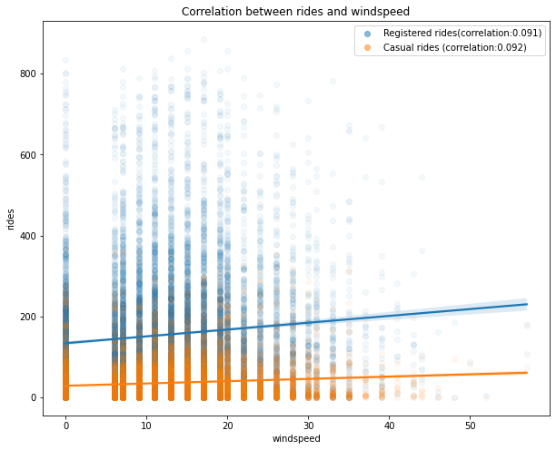
Correlation between the number of rides and the wind speed
Correlation Matrix Plot
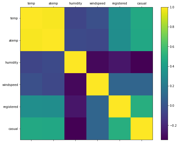
The conclusion of the visualization is that when the temperature is good the hire of the bike is good for both registered users and casual users.
Training After adding additional features
predictor_new_features = TabularPredictor(label="count",
                             eval_metric='root_mean_squared_error',
                             problem_type='regression',
                             learner_kwargs={'ignored_columns': ['casual','registered']}
                            ).fit(train_data=train,
                                  time_limit=600,
                                  presets="best_quality"
)
The model performed better after changing some of the columns/features to categorical data and also after adding new features.
Training Hyper parameter tuning
num_trials = 5
search_strategy = 'auto'
hyperparameters = {
  'NN_TORCH': {'num_epochs': 10, 'batch_size': 32},
  'GBM': {'num_boost_round': 20}
}
hyperparameter_tune_kwargs = {
  'num_trials': num_trials,
  'scheduler' : 'local',
  'searcher': search_strategy,
}


predictor_new_hpo = TabularPredictor(label="count",
                             eval_metric='root_mean_squared_error',
                             problem_type='regression',
                             learner_kwargs={'ignored_columns': ['casual','registered']}
                            ).fit(train_data=train,
                                  num_bag_folds=5,
                                  num_bag_sets=1,
                                  num_stack_levels=1,
                                  time_limit=600,
                                  presets="best_quality",
                                  hyperparameters=hyperparameters,
                                  hyperparameter_tune_kwargs=hyperparameter_tune_kwargs
)
After hyperparameter tuning, the model slightly changed from the kaggle score of 1.33 to 1.32
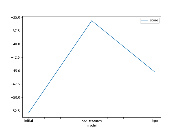
A line plot showing the top model score for the three (or more) training runs during the project.
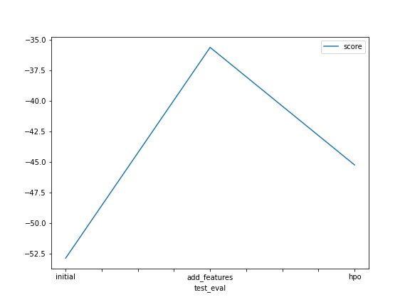
Create a line plot showing the top kaggle score for the three (or more) prediction submissions during the project.
Summary
Estimated performance of each model:
                             model   score_val  pred_time_val    fit_time  pred_time_val_marginal  fit_time_marginal  stack_level  can_infer  fit_order
0              WeightedEnsemble_L3  -45.237593       0.001964  136.536450                0.000992           0.555725            3       True         14
1   NeuralNetTorch_BAG_L2/877bc604  -45.947510       0.000861  124.461472                0.000160          32.741020            2       True         13
2               LightGBM_BAG_L2/T5  -49.723478       0.000812  103.239705                0.000111          11.519253            2       True         12
3              WeightedEnsemble_L2  -51.955120       0.001266   46.451789                0.000971           0.569900            2       True          7
4   NeuralNetTorch_BAG_L1/469e5854  -56.261557       0.000171   34.386352                0.000171          34.386352            1       True          6
5               LightGBM_BAG_L2/T2  -61.015430       0.000808  103.493750                0.000107          11.773299            2       True          9
6               LightGBM_BAG_L1/T5  -62.269851       0.000124   11.495537                0.000124          11.495537            1       True          5
7               LightGBM_BAG_L1/T2  -70.588170       0.000097   11.423693                0.000097          11.423693            1       True          2
8               LightGBM_BAG_L2/T3  -77.938179       0.000776  103.443859                0.000075          11.723408            2       True         10
9               LightGBM_BAG_L2/T1  -78.093263       0.000785  103.862269                0.000084          12.141818            2       True          8
10              LightGBM_BAG_L1/T3  -90.207152       0.000110   11.416231                0.000110          11.416231            1       True          3
11              LightGBM_BAG_L1/T1  -95.483677       0.000120   11.565247                0.000120          11.565247            1       True          1
12              LightGBM_BAG_L2/T4 -161.546488       0.000813  103.448732                0.000112          11.728281            2       True         11
13              LightGBM_BAG_L1/T4 -165.490162       0.000080   11.433391                0.000080          11.433391            1       True          4
Number of models trained: 14
Conclusion
- Initial Training
The training time takes is very long compered to when feature engineering was applied There was no data preprocessing in the initial stage of training which is good feature
- New features Training
The score was improved as well as the training time. The new features which were added during feature engineering enhaced the model training fro better results
- Hyperparameter Tuning Training
The time for training was a lot faster compared to the other stages. The number of models for training were 14 compared to 15 with the default parameters.
AutoML frameworks offer an enticing alternative. For the novice, they remove many of the barriers of deploying high performance ML models. For the expert, they offer the potential of implementing best ML practices only once (including strategies for model selection, ensembling, hyperparameter tuning, feature engineering, data preprocessing, data splitting, etc.), and then being able to repeatedly deploy them. This allows experts to scale their knowledge to many problems without the need for frequent manual intervention.
Reflection
Many models are better than few and hyperparemeter tuning enhances learning. There is no train split manually the model does that internally. The model handles missing values and this is the second stage during training
I will spend more time doing the data analysis to get to know data in detail trying different analysis methods.